In part 1, we laid down the foundation for band trading by reviewing the concept of trend and trend analysis. In this article, we will study some popular bands and channels. We’ll also analyze how bands can improve the reliability of signals without altering the overall trend profile and how they could be used to slow down trading without sacrificing the biggest profits. The time of greatest indecision is the point of trend change, when traders get whipsawed the most. A simple way to avoid frequent false signals is by using a band.
The original Keltner Channel, named after Chester W. Keltner who was a Chicago based corn trader, is not in use today. Keltner used a ten-day simple moving average of typical price, TP=(High+Low+Close)/3, as the center line and built a band around it by plotting a line above it using the simple moving average of highs and a line below using SMA of lows. All three simple moving averages used the same look back period of 10 day. The modern Keltner channel uses either SMA or EMA (Exponential Moving Average) for the centerline and Wilder’s ATR (Average True Range) multiplied by a volatility factor to create the bands.
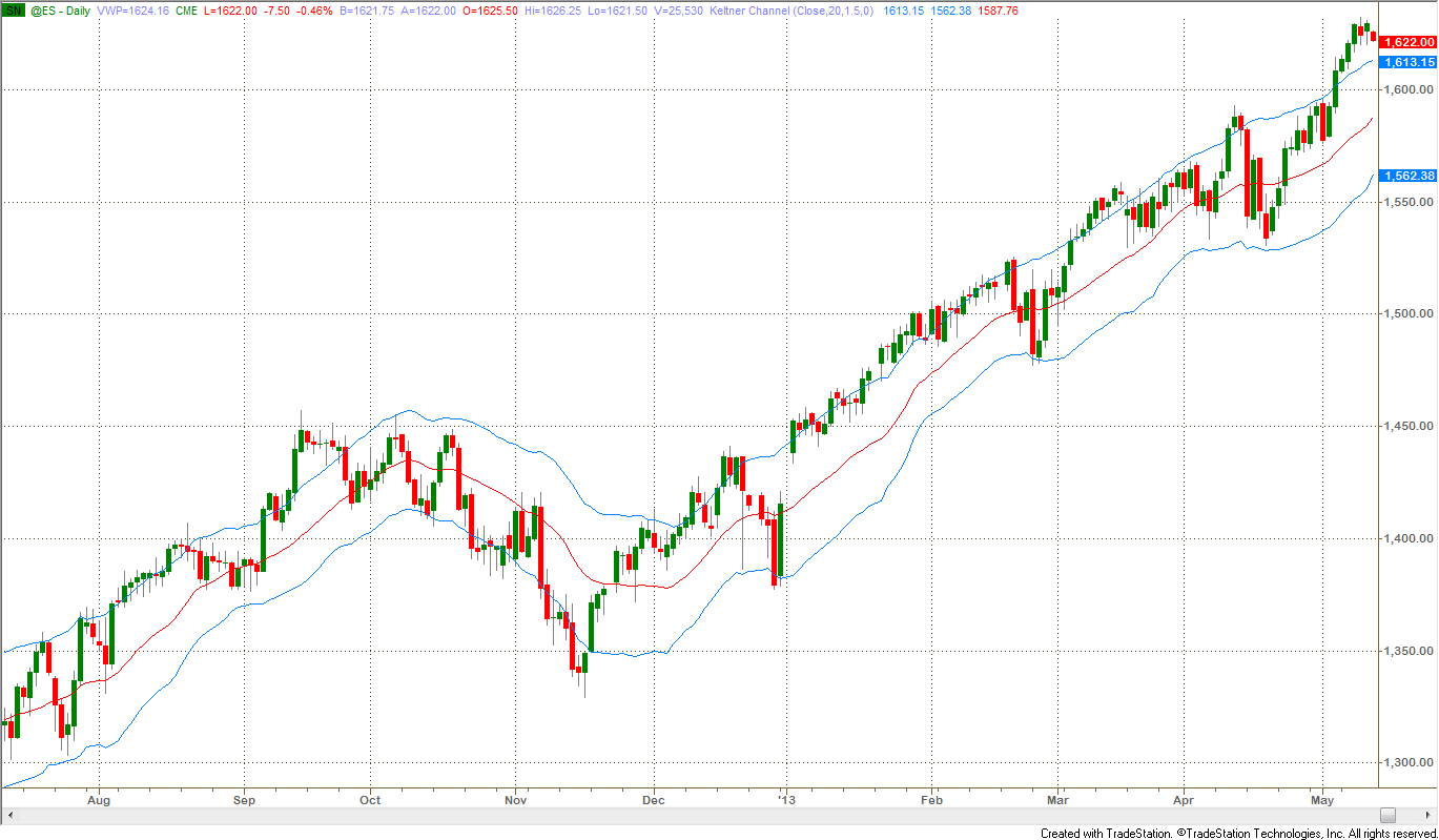
Figure 1 shows Keltner Channel applied to the chart of S&P500 e-mini futures.
Figure 1: Keltner Channel plotted on a 9-Month Daily Charts of ES
Keltner channel is used in two ways:
- to identify breakouts for trend following, and
- to find overbought/oversold price levels within trading ranges.
The problem with using ATR is its slow response to changes in volatility. Creating a band that is responsive to volatility can improve the reliability of trend signals and there are many methods from which to choose though all of these methods use a constant value as a multiplier or scaling factor for scaling.
The volatility multiplier or factor increases or reduces the sensitivity of the band to changes in price. In simple mathematics, if s is a scaling factor and p is a fixed percentage, then the following bands can be constructed:
- Percentage of Trendline Band = MA ± s x p x MA
- Percentage of Price Band = MA ± s x p x Price
- Average True Range Band = MA ± s x ATR of previous bar x MA
- Standard Deviation Band = MA ± s x STDev of previous bar x MA
In the above formulas, MA is the moving average of price and Band is the value calculated for plotting the band on the price chart. To calculate both bands (up and down from the MA), two values must be calculated using +s and –s, therefore ±s.
A robust measurement of price volatility is the standard deviation of the price itself, calculated over a period of recent price history, which is the last formula, listed above. John Bollinger popularized the combination of a 20-day simple moving average with bands formed using 2 standard deviations of price changes over the same 20 day period and they are now frequently called Bollinger Bands.
Because the standard deviation represents a confidence level, and prices are not normally distributed (i.e. due to fat tails in price action of financial markets), the choice of two standard deviations produces an 87% confidence band. If prices were normally distributed, two standard deviations would have equated to 95.4% of the price action range. Trading systems based on Bollinger bands are usually combined with other techniques to identify extreme price levels.
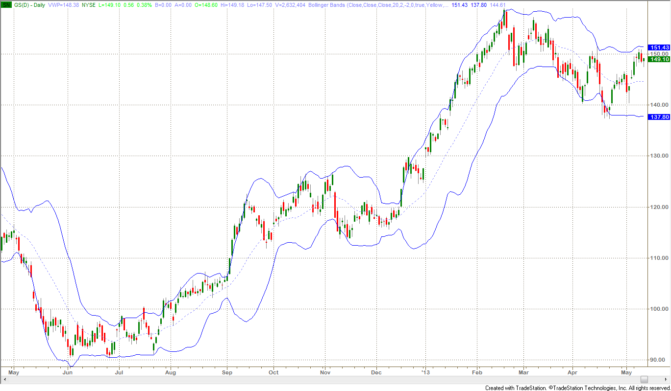
Figure 2: Standard Bollinger Bands on a One-Year Daily Charts of GS
Simple Moving Average 20, ±2 Standard Deviations
Characteristically, once the price moves outside either the upper or lower Bollinger Band, it remains outside for a number of days in a row. This type of behavior is called “crawling up the bands” and is typical of what is also called “high momentum”. Note that the width of the band varies considerably with the volatility of prices and that a period of high volatility causes a “bubble”, which extends past the period where volatility declines. Bollinger bands are excellent for showing the cyclical nature of volatility: low volatility begets high volatility and vice-versa. It is also possible to apply Bollinger bands to different time frames to clarify major and minor trends in the market as in the chart below which combines weekly and daily bands.
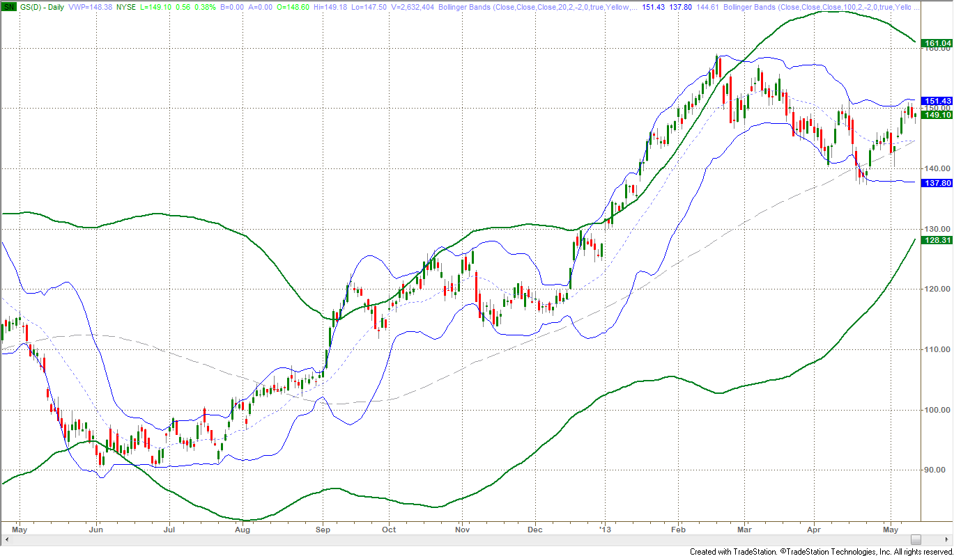
Figure 3: One-Year Daily Chart of GS with Standard Bollinger Bands
Blue: Daily Bollinger Bands, Green: Weekly Bollinger Bands
This is the same chart of Goldman Sachs (GS) with both daily and weekly Bollinger bands plotted on the same daily bars. It clearly shows how the higher time frame, weekly Bollinger bands influence and contain the lower time frame, daily Bollinger bands. Notice the high momentum trend that started in early 2013, put price bars outside the weekly band and kept them there for two months though the daily Bollinger Bands still contained the price bars. The weekly bands puts the move in the proper context of momentum which might otherwise be indistinguishable.
Any volatility measure based on historic data including Bollinger Bands, expand quickly after a volatility increase but are slower to contract as volatility declines. The Achilles heel of Bollinger bands is the time it takes for them to contract after volatility drops off, which makes trading some instruments using Bollinger bands alone difficult or less profitable. You would need other techniques in a conventional Bollinger band system to make it workable.
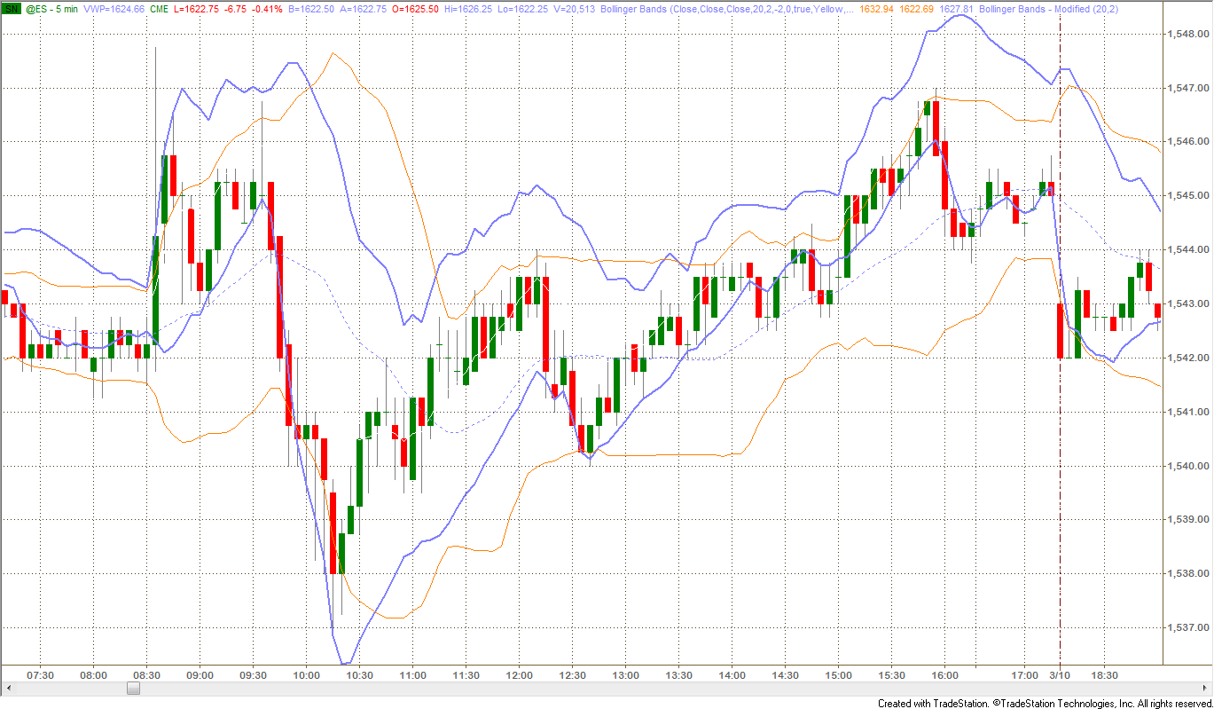
The chart below illustrates this problem:
- Point 1: Bands quickly expand as volatility expands.
- Point 2: Bands do not contract quickly enough to give the trader the famous squeeze pattern to trade a reversal. Traders must use another indicator to find the first reversal up from the bear move or simply skillfully read the price action.
- Point 3: The squeeze finally comes, but half of the bull reversal move has happened already. If you consider the first small squeeze (before point 2), two-thirds of the move was missed by the time the squeeze forms.
Figure 4: Standard Bollinger Bands on a 5-Min Intraday Chart of ES (March 8, 2013)
Notice the slow contraction of these bands incurs delay in trader’s decision making
It is possible to correct this problem. Dennis McNicholl wrote about a new method for calculating Bollinger bands in an article: “Better Bollinger Bands” (Futures magazine, October 1998). McNicholl recommends adjusting Bollinger Bands by modifying
- the center line formula and
- different equations for calculating the bands,
so that they follow price more closely and respond faster to changes in volatility. *See code below
The chart below compares the two Bollinger bands on the same 5-min intraday chart of the ES futures contract. Heavier blue lines are the modified bands.
Figure 5: 5-Min Intraday Chart of ES (March 8, 2013) with both Modified and standard Bollinger Bands:
notice the fast response of modified bands compared to standard ones
We built upon the concept of trend from part 1 and discussed some of the more popular trading bands and core techniques for trading them in this article, except one. The most complex and advanced band construction technique is based on statistics rather than factors of price only. Part 3 is dedicated to this subject.
*The following short code for TradeStation plots a modified Bollinger band based on McNicholl’s formulas (from “Better Bollinger Bands” by Dennis McNicholl, “Futures,” October 1998):
//--- Modified Bollinger Bands ---
Inputs:
INT period(20),
Double factor(2.0);
Variables:
alpha(0),
m1(0),
ut(0),
dt(0),
m2(0),
ut2(0),
dt2(0),
but(0),
blt(0);
//--- Smoothing Constant ---
alpha = 2/(period + 1);
mt = alpha*close + (1 – alpha)*m1;
ut = alpha*m1 + (1 – alpha)*ut;
dt = ((2 – alpha)*m1 – ut)/(1 – alpha);
mt2 = alpha*absvalue(close – dt) + (1 – alpha)*m2;
ut2 = alpha*m2 + (1 – alpha)*ut2;
dt2 = ((2 – alpha)*m2 – ut2)/(1 – alpha);
but = dt + factor*dt2;
blt = dt – factor*dt2;
//--- Plot Bands ---
plot1(dt,”center”);
plot2(but,”upper”);
plot3(blt,”lower”);
//--- End of Indicator: Modified Bollinger Bands ---